My file organization: Directory: “R Course”, Project: “Organizing Data”, File: “Data Cleaning”
In this course, we will be using the “iris” dataset built into R, so we don’t need to load a data file. BUT if you need to load your own data, make sure your .csv file is in your Directory (The folder that you made on your computer and then set as Directory in R Studio) and load your file:

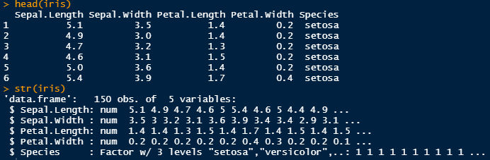
Let’s take a quick look at our data. We can do this with a few functions:
head() – this function shows you the first few rows of your data
str() – this functions shows you the structure of your data (eg. which columns are numerical or logistic, etc)
Here are some common data types (structures) and their examples:
- logical: yes/no; true/false
- numeric: -infinity to +infinity (including decimals)
- integer: -infinity to +infinity (full numbers only, no decimals)
- character: colours, countries, types of plants
So if we take a look at the structure of “iris” we can see that 4 columns are numerical and one column is a factor (similar to character) limited to 3 “levels” – so only 3 categories.
Structure will also show you if you’ve made some spelling mistakes or typos if it categorizes your column wrong. For example it states that a column is a character, when you know for sure it is all numbers. Perhaps you accidentally typed in a letter in that numerical column? Or if you have a character value with 3 levels, but R str() is showing that you have 4 levels, most likely you’ve misspelt one of the variables or just added a capital letter – R is very specific with capital letters.
Let’s “clean” our data
Here are a few simple functions you can do to check your data:
Duplicates:
- sum(duplicated()) – how many duplicated rows are in your data
- duplicated() – which row, indicated by TRUE, is duplicated in your data
- distinct() – creates a new dataset with the duplicated row removed

Data Structure:
Sometimes you may need to change the structure of your data. For example you’ve loaded your data file and R thinks your numerical column is an integer, but you’d rather treat it as a numerical value. You can always check what structure your column is in by typinf “is.FORMATOFDATA” and then converting it with “as.TYPEOFDATAYOUWANT”
For example:

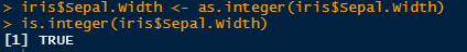
Did you notice how I had to use “iris$Sepal.Width” first? Let’s break this down.
iris: telling R which data file to change
$Sepal.Width: telling R which column within the data file to change
If I wanted to add an extra column where the data is formatted differently I would do this:

Adding extra columns with your raw data transformed is common and is a better practice than changing the raw data directly.
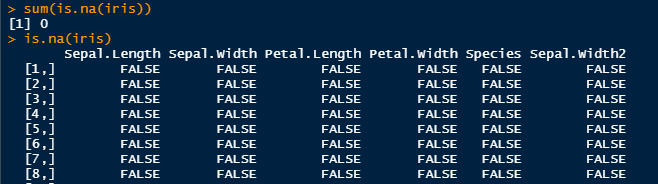
Finding NA values in your Data:
- sum(is.na(YOURDATA): How many NA values are in your data file?
- is.na(YOURDATA) : are there any NA values in your data file, if so which row?
There are many reasons for having NA values in your data. For example, you were doing field work and you couldn’t go outside to collect data due to weather one day, or the test tube you were using with a sample slipped and broke. Things happen!
How you treat NA values is different depending on why the NA values occurred and how many NA values you have. Most statistical analyses, graphs, etc, will run with NA values present in your data, so I typically encourage people to keep NA values in.
If you insist on removing NA values you can use:
- na.omit(DATA): omit the NA values. This will remove full rows with the NA value.
But please do this with caution, and always consult a supervisor, mentor, or stats consultant to see if it is ok for you to remove the NA values. Removing data, even NA’s, can cause more harm than good.
